Group Pivot Table Numbers by Tens

Instead of showing a long list of items in a pivot table, you can group dates or numbers, and even text, to create a shorter list.

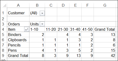
In this example, the units have been grouped by tens, so there are only 5 columns of summarized data, instead of 50.

pivotgroupnumbers01

The starting number for the grouping has been set at 1, and the upper limit has not been set. If higher number are added to the source data, those number would appear in new groupings.

Watch the Grouping Video

To see the steps for grouping numbers, you can watch this short video tutorial.

Download the Sample File

For more information on grouping data in a pivot table, and to download the sample file, please visit my Contextures website: Pivot Table Grouping

_________

Show Subtotals at Bottom of Pivot Field

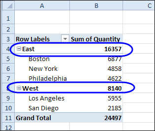
When you add fields to the Row Labels area of a new pivot table, subtotals are automatically shown at the top of each group of items, for the outer fields.

subtotalstop01

You can turn the subtotals off, or move them to the bottom of the group, if you prefer.

Watch the Video

To see how to add subtotals, and move them, you can watch this short video tutorial. You’ll also see how the pivot table’s report layout affect the subtotals in the Row Labels area.

For written instructions, and more details on working with subtotals, please visit my Contextures website: Pivot Table Subtotals

_________________________

Grouped and Ungrouped Dates from Same Pivot Table Source

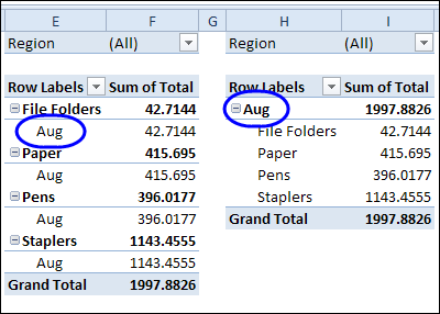
In some workbooks, you might create two or more pivot tables that are based source data. Even if they are on different worksheets, those pivot tables will share some features, such as calculated items and grouped fields.

pivotcacheshared01 

So, if you group the dates in one pivot table, the same grouping will show up in the other pivot table. This occurs because the pivot tables share the same pivot cache. You can manually create a separate pivot cache, by copying one of the pivot tables to a different workbook, temporarily. See the instructions here.

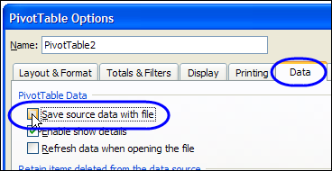
Note: If you create a separate pivot cache for one of the pivot tables, the file size might increase substantially. To reduce the effect, you can turn off the option to save the source data with the file.

pivottableoptionssavedataoff 

Create New Pivot Cache with VBA

Instead of manually creating a separate pivot cache for a pivot table, you can select a cell in the pivot table, and run the following code.

It adds a temporary sheet to the workbook, and creates a new pivot table there, based on the same data source, but in a new pivot cache. The selected pivot table is set to the same pivot cache as the new table, and then the temporary sheet is deleted.

Sub SelPTNewCache()
    Dim wsTemp As Worksheet
    Dim pt As PivotTable
    
    On Error Resume Next
    Set pt = ActiveCell.PivotTable
    
    If pt Is Nothing Then
        MsgBox "Active cell is not in a pivot table"
    Else
        Set wsTemp = Worksheets.Add
        
        ActiveWorkbook.PivotCaches.Create( _
            SourceType:=xlDatabase, _
            SourceData:=pt.SourceData).CreatePivotTable _
            TableDestination:=wsTemp.Range("A3"), _
            TableName:="PivotTableTemp"
        
        pt.CacheIndex = wsTemp.PivotTables(1).CacheIndex
        
        Application.DisplayAlerts = False
        wsTemp.Delete
        Application.DisplayAlerts = True
    End If
    
exitHandler:
        Set pt = Nothing

End Sub

_____________________

Change Excel Pivot Table Subtotal Text

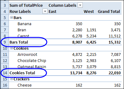
When you add two or more fields to the Row area in a pivot table, the outer fields will automatically display subtotals. By default, the subtotal row has a label that stars with the item name, followed by "Total"

In the pivot table shown below, the Category and Product fields are in the Row Labels area, and there is a subtotal for each item in the outer field – Category. You can see the Bars Total and Cookies Total labels.
pivotsubtotaltext01

Instead of leaving the default subtotal labels, you type a new label in any subtotal row. The text that you enter will apply to all the subtotals in that field.

Type a New Subtotal Label

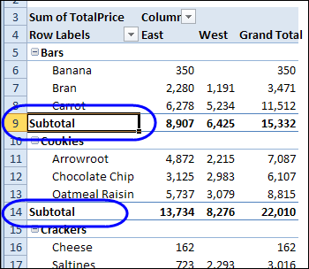
When you type a new subtotal label, you can include the item name, or omit it. For example, if you select the Bars Total label in cell A9, and type "Subtotal", all of the items will change to that label. There is no item name in any subtotal label.
pivotsubtotaltext02

Include the Item Name

If you include the item name, such as Subtotal – Bars, when typing the new text, each subtotal will include its own item name.
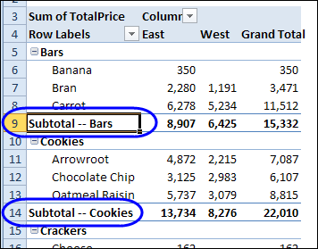
pivotsubtotaltext03

When you type the item name, be sure to type it exactly as it appears in the pivot table. If you misspell the item name, such as "Bar" instead of "Bars", that word will be included in all the other subtotal labels.
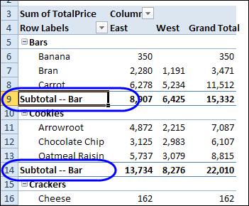
pivotsubtotaltext04

Text Before and After Item Name

You can add text before and/or after the item name in the subtotal label. In the next example, the Bars subtotal label was changed to, "This is the Bars Subtotal". The other products show the same text before and after their item names.
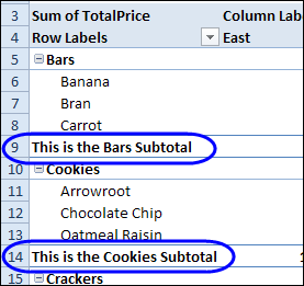
pivotsubtotaltext07 

Get Creative with Subtotals

In addition to text, you can use other characters in the subtotal labels. In the example below, I typed a couple of space characters, then equal signs and a greater than symbol, to create an arrow.
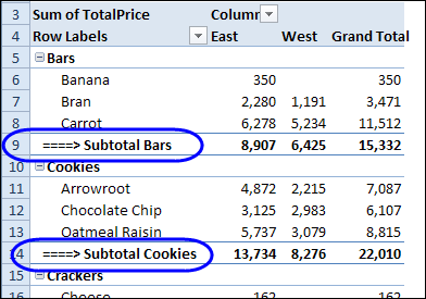
pivotsubtotaltext05 

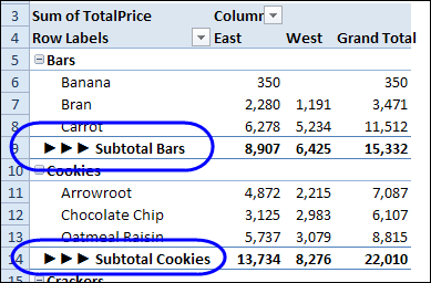
In the next example, I pressed the Alt key, and typed 16 on the numeric keypad, to create a right-pointing triangle. That certainly draws attention to the subtotals!
pivotsubtotaltext06 

NOTE: If you’re using a keyboard that doesn’t have a separate numeric keypad, you might have to press the Fn key, and the Alt key, then type 16 on the numbers that appear on the JKL keys.

So, you can get creative with those subtotal labels. Just remember that they can’t be changed individually – a change to one will be applied to all of them.

_____________________
Pivot Table Grand Totals at Top

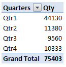
When you create an Excel pivot table, the grand totals are automatically added at the bottom, and at the right. With the Grand Total command on the Excel Ribbon, you can show or hide the grand totals, but you can’t move them.

The good news is that there is a quick and easy workaround for this problem, which allows you to show the column grand total at the top.

There are written instructions on my Contextures website, on the Pivot Table Grand Totals page, where you can also download a sample file for this technique.

Watch the Grand Totals Video

To see the steps for the grand total workaround, please watch this short video.

__________________

Quickly Remove Pivot Table Grand Totals

You probably know how easy it is to add or remove the Grand Totals in a pivot table, by using the Ribbon commands.

But keep reading, to see an even quicker way!

Grand Totals on the Ribbon

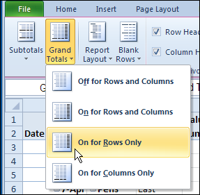
Yes, it’s easy to change the Grand Total settings on the Ribbon:

  • Select any cell in the pivot table
  • On the Ribbon, under PivotTable Tools, click the Design tab
  • In the Layout group, at the left, click Grand Totals
  • Click one of the options.

GrandTotalRemove01

Quickly Remove Grand Totals

For an even quicker way to remove Grand Totals, follow these steps:

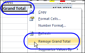
  • In the pivot table, right-click the Grand Total label cell (not the total amounts) – either the Row Grand Total or the Column Grand Total
  • In the popup menu, click Remove Grand Total

GrandTotalRemove02 

That’s it! Unfortunately, there’s no equally quick way to add Grand Totals, but maybe that feature will be in the next version of Excel.

________

Pivot Table Grouping Affects Another Pivot Table

pivotgroupcache00In Excel 2007, when you create a second pivot table from the same source data, you don’t get an option to base the new pivot table on an existing pivot table, the way you can in Excel 2003.
In Step 1 of the Excel 2003 Wizard, you can select the first option, to create an independent pivot table. Or, select the fourth option, for pivot tables that share the same pivot cache.

pivotgroupcache02

In Excel 2007, if you create two pivot tables from the same source data, they automatically use the same pivot cache of the source data. You don’t have an option to create an independent pivot table.

Grouping Problems

Because the pivot tables share the same cache, this can cause problems if you group the data in the pivot fields.

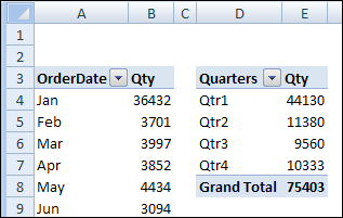
When you change the grouping in one pivot table, the same grouping appears in the other pivot table. For example, change the date grouping in the first pivot table to Months, and the dates in the second pivot table automatically group in Months.

Because you created the two pivot tables from the same source data, by default they use the same pivot cache, which is where the grouping is stored.

However, you might want different grouping in the two pivot tables. For example, you’d like Month grouping in one pivot table, and Quarter grouping in the other.

pivotgroupcache01

Create a Second Pivot Cache

To use different grouping in each pivot table, you’ll need to create a separate pivot cache for each pivot table. Use the following easy method, suggested in the Excel newsgroups by Dave Peterson.

To create a separate pivot cache for the second pivot table:

  1. Cut the second pivot table, and paste it into a new workbook.
  2. Change the grouping of the second pivot table.
  3. Cut the second pivot table from the new workbook, and paste it back into the original workbook.

Now there are two pivot caches in the original workbook, and each pivot table can be grouped independently.

Watch the Video

To see the steps for creating a second pivot cache so you can create separate grouping in the pivot tables, please watch this Excel video tutorial.

________________

Grouping Pivot Table Dates by Months and Weeks

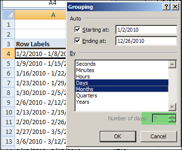
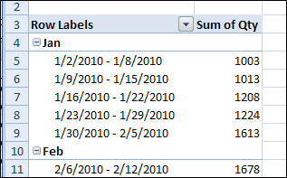
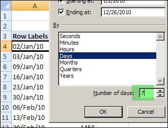
In a pivot table, there’s no built-in way to group the pivot table data by both weeks and months at the same time. If you want to show sales data by week, you can group the date field in seven-day intervals.

groupweekmonth01

The 7 day grouping works well, but if you try to add grouping by months, the Number of Days option is disabled. If you select Month in the Grouping dialog box, the days will lose their 7 day grouping.

groupweekmonth02

Calculate the Month

Since you can’t group by both week and month, you can use a workaround instead. You could create a column in the source data, and then calculate one of the grouping levels there. Then, you could add that field to the pivot table.

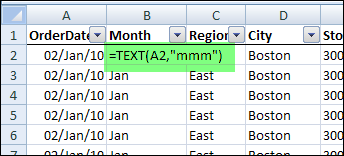
For example, you can add a column that calculates the month name for each sales order date, by using the TEXT function:

=TEXT(A2,"mmm")

groupweekmonth03

Add the Month field to the pivot table, above the weeks.

groupweekmonth04

Calculate the Week Number

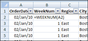
Another option is to add a column to the source data, with a formula to calculate the week number:

=WEEKNUM(A2).

groupweekmonth05

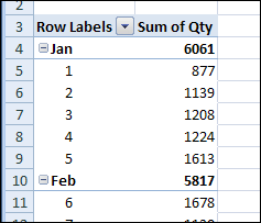
With the OrderDate field in the Row Labels area, group the dates by months. In the Row Labels area, add the WeekNum field below the OrderDate field, to summarize the data by month and week number.

groupweekmonth06

Note: If a week begins in one month and ends in another, it will appear under both months.

________________

Change Summary Function for Pivot Table Subtotal

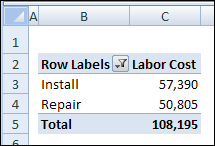
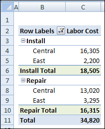
When you add a field to the Values area of an Excel Pivot Table, it automatically shows the Sum or Count for all the items in that field. Here we can see the total labor cost for each Service Type.

pivotsubtotal00

If you add more than one field to the Row Labels or Column Labels area of the Pivot Table, a subtotal is automatically created for each field except the last one (the Inner Field). The subtotal, by default, uses the same summary function as the Value field.

In our example, the District field has been added to the Row Labels area. Service Type is now an Outer Field, and has a subtotal for each service. District is the Inner Field, and does not have subtotals.

pivotsubtotal01

Change the Subtotal Summary Function

Instead of using the default summary function for subtotals, you can select a different function. To change the setting:

  1. Right-click a label for the field in which you want to change the subtotal. In this example, right-click cell B3, which has the Install label.
  2. In the pop-up menu, click Field Settings
  3. In the Field Settings dialog box, click the Subtotals & Filters tab
  4. Under Subtotals, click Custom
  5. In the list of Summary Functions, click one or more function names
  6. Click OK to close the dialog box.

Subtotals on Inner Fields

For the Inner Field in the Row Labels or Column Labels area, the default subtotals are not displayed. So, in the pivot table shown above, there’s no subtotal for the District field.

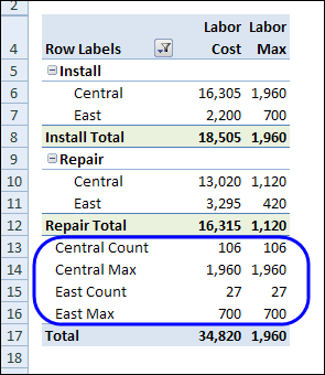
However, if you create Custom Subtotals for an Inner Field, those subtotals appear at the end of the Pivot Table. In this example, Custom subtotals for Count and Max were created for the District field. You can see the District subtotals at the bottom of the Pivot Table, just above the Grand Total.

pivotsubtotal04

More Info on Pivot Table Subtotals

You can read more about pivot table subtotals, and the steps for changing them, on the Contextures website: Excel Pivot Table Subtotals.

Watch the Pivot Table Subtotals Video

To see the steps for changing the pivot table subtotals, and creating multiple subtotals, you can watch this short video.

___________