When you set up a pivot table, the outer field names each appear once, at the top of the group. In the screen shot below, The category names are in the left column, and the products for each category are listed below the headings.
Show Repeating Labels
In Excel 2010, and later versions, you can change a pivot field setting, to show the field names in every row, instead of just once. This is useful if the the lists are long, and you can’t see the headings as you scroll down. You can also do lookups from the pivot table, if the names are filled in.
A pivot table is a great way to see a summary of sales to your customers. You can see how much they bought, and how much they spent, on each product. In the pivot table below, each customer is listed, and below the customer name is a list of products and quantities.
When you set up a pivot table, there might be a few blank cells in the Values area. In the example below, no Banana Bars were sold at stores 3062 or 3659.
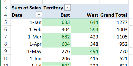
You can apply conditional formatting rules to a pivot table, just as you would in other cells on a worksheet. In the screen shot below, cells with amounts above average are filled with light green.
It’s a little thing, but it can be frustrating if your pivot table column widths keep changing. In the screen shot below, I’ve made column B narrow, so the pivot table takes up less room across the worksheet.
But, when I select a customer name, instead of showing all the customers, the column width adjusts to fit the selected name.
Now, column B is much wider, and it’s hard to read the numbers in that column, because they’re off to the right of the heading.
This automatic adjustment of the column width is useful sometimes, but for other pivot tables, where the column layout is fairly static, it’s not so helpful!
Change the Autofit Setting
If you have adjusted your pivot table column widths, and you want them to stay that way, you can change a setting in the pivot table options.
Right-click any cell in the pivot table, and click PivotTable Options
In the PivotTable Options window, click the Format tab
In the Format section, remove the check mark from Autofit column widths on update
Click OK, to close the PivotTable Options window.
With the Autofit setting turned off, the column widths will stay the where you set them.
If you want the Autofit feature back on at any point, go back to the PivotTable Options, and add a check mark for Autofit columns.
____________
When you add fields to the value area in a pivot table, custom names are automatically created, such as Sum of Quantity or Count of Customer.
Excel won’t let you remove the “Sum of” in the label, and just leave the field name. However, you can change the heading to the field name, plus a space character, to work around this problem.
In the screen shot below, the heading has been changed to [space]Qty.
Change (Blank) Labels
Another formatting fix that you can make is to get rid of the labels that say “(Blank”)”. These appear if cells are blank in the source data, and you add those fields to the row or column labels area.
Excel shows an error message if you just try to delete those labels, but you can use a space character to replace them.
Watch the Video
Watch this short video tutorial to see how to make these changes to the pivot table headings and labels.
In a pivot table that contains a long list of dates, you can use conditional formatting to highlight a specific date range. In this example, the pivot table contains forecast data for 2.5 years, with dates in the OrderDate field.
When the file opens, we’re usually interested in checking the forecast amounts for the upcoming month. It can take a bit of time and concentration to find those dates in the long list. We’ll highlight the labels in yellow, so they stand out, and are easy to find.
We’ll use dynamic conditional formatting (Next Month), so the highlighting will change each month when we open the workbook.
Highlight the Upcoming Month
Follow these steps to highlight Row Labels where the order forecast date is in the upcoming month. It’s currently August, so the September dates will be highlighted.
In the pivot table, remove any filters that have been applied – all the rows need to be visible before you apply the conditional formatting.
Select all the dates in the Row Labels that you want to format.
On the Ribbon, click the Home tab, and then in the Styles group, click Conditional Formatting.
In the list of conditional formatting options, click Highlight Cells Rules, and then click A Date Occurring.
In the date range drop-down, select Next Month, and then click the arrow to open the formatting drop-down list.
Select one of the formatting options, or create a Custom Format. I selected Custom Format, and used a yellow fill colour.
Click OK to close the A Date Occurring dialog box.
The dates from the upcoming month are highlighted, and will stand out in the report when you open the workbook.
Conditional Formatting Warnings
This pivot table’s source data won’t change, because we don’t alter the forecast after it has be finalized.
However, if you apply conditional formatting to a pivot table, and new data is added, it might not be included in the formatted area. Be sure to check the range, in the Manage Rules box for Conditional Formatting, and edit the rule, if necessary.
Also, if you change the location of the date field, the conditional formatting will not automatically move with that field. You will have to modify the conditional formatting rule, to point to the new location.
In Excel 2003, and earlier versions, when you added multiple data fields to a pivot table, they were automatically arranged vertically. The data headings showed up in the Row area, stacked one on top of the other.
Here is the same pivot table, with horizontal data headings.
Vertical Data in Excel 2010 Pivot Table
Pivot tables changed quite a bit in Excel 2007, and the default layout for multiple data fields is now horizontal. Using the same data, this is the default layout in Excel 2010.
If you want to change the data to a vertical layout, you can drag the Values button in the Pivot Table Field List, from the Column Labels area to the Row Labels area.
Usually, the Values button would be positioned below the other fields in the Row Labels area.
After you move the Values label, the data fields will be rearranged, and they will show vertically, with headings in the Row Labels area.
Watch the Excel 2010 Data Layout Video
To see the steps for rearranging the data in Excel 2010, please watch this short video tutorial.