Long ago, there was a Chart Wizard in Excel, and it had some built-in Combination Chart Types, like Column-Line. The Chart Wizard disappeared in Excel 2007, along with the combo chart type options.
You could still create combo charts in Excel 2007 and 2010, but it wasn’t quite as obvious how to do that.

Combo Charts in Excel 2013
In Excel 2013, it’s easier to change a chart to a combo chart.
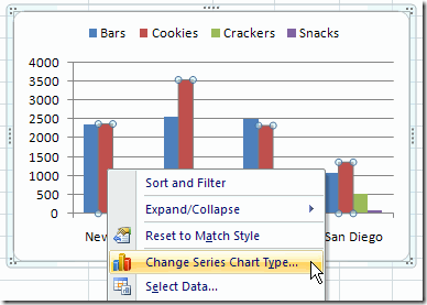
- Right-click on the chart, and click Change Chart Type
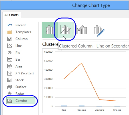
- At the left, select Combo as the category
- At the top, select one of the built-in combo types, or click the last option, to create a custom combo type.

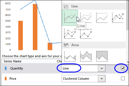
- At the bottom, you can change the chart type for any series, and select which series to plot on a Secondary axis.

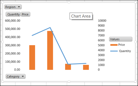
- Click OK when you’re finished, to see the completed chart on the worksheet.

Download the Sample File
You can download the sample file for this tutorial from my Contextures website: Pivot Chart Tutorial
Watch the Video
To see the steps for creating a pivot chart, and changing it to a combination column-line chart, please watch this short video.
Or watch on YouTube: Create Column Line Chart for Excel 2013 Pivot Table
____________________________

One thought on “Combo Column Line Pivot Chart in Excel 2013”