Create Pivot Chart from Data in Excel 2013

With a new feature in Excel 2013, you can create a pivot chart right from the source data – you don’t have to build a pivot table first.

You can watch this short video tutorial, to see how it works, and the written instructions are below the video.

Create a Pivot Chart from the Data

Follow these steps to create a pivot chart in Excel 2013.

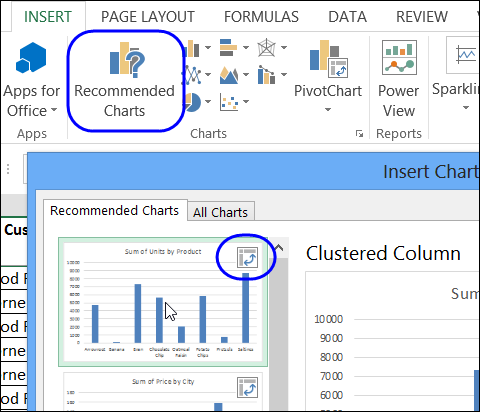
1. Select a cell in the source data, and on the Ribbon, click the Insert tab.
2. Click Recommended Charts, then scroll through the list of options.
3. Some of the charts have a pivot table symbol at the top right — click one of those to create a pivot chart.

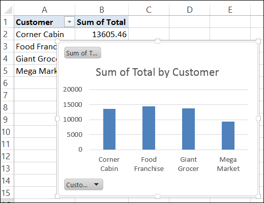
A new sheet is added to the workbook, with pivot chart that you selected, and its connected pivot table.

_______________________