There is a new feature in Excel 2013, that makes it even easier to get started with pivot tables.
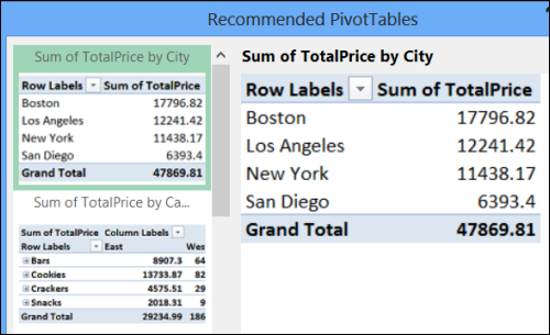
Just select a cell in your source data table, and on the Ribbon’s Insert tab, click Recommended PivotTables.

A window opens, and you can see a list of suggested pivot table layouts, based on your data.

Click on any layout, to see a larger view of it, and when you select one that you want to use, click the OK button.
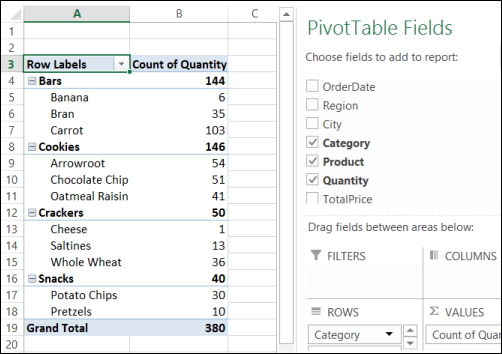
Your pivot table is created on a new worksheet, and you can leave it as is, or make changes to it.

Watch the Video
To see the steps for creating a pivot table in Excel 2013, please watch this short video tutorial.
Download the Sample File
To download the sample file for this video, please visit my Contextures website: Create a Pivot Table
__________________
