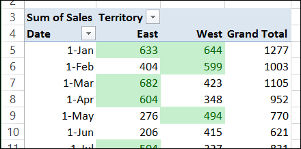
You can apply conditional formatting rules to a pivot table, just as you would in other cells on a worksheet. In the screen shot below, cells with amounts above average are filled with light green.

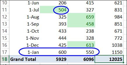
However, if you change the pivot table layout, or add new data, the correct cells might not be formatted. In the screen shot below, a new month’s data was added, and those cells are not formatted.

Change the Formatting Range
To prevent this problem, you can adjust the formatting rules, so they refer to the pivot fields, instead of a specific range of cells.
- Select a pivot table cell, and on the Ribbon’s Home tab, click Conditional Formatting, then click Manage Rules
- Select your pivot table rule, and click Edit Rule, to open the Edit Formatting Rule window.
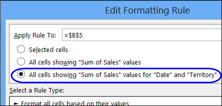
- In the Apply Rule To section, there are 3 options, and the Selected cells option is selected.
- The Selected cells option works in many cases, but may not adjust correctly if the layout changes
- All Cells Showing “Sum of Sales” Values might include too many cells, such as subtotals, and Grand Totals
- All Cells Showing “Sum of Sales” Values for “Date” and”Territory,” is the best option for this pivot table. It formats cells where the Date and Territory values appear, and excludes subtotals and Grand Totals
- Click on the 3rd option — All cells showing “Sum of Sales” values for “Date” and “Territory”, then click OK

The conditional formatting automatically adjusts, to include the new month’s data.

Watch the Video
To see the steps for applying the conditional formatting and changing the data range setting, please watch this short video tutorial.
Download the Sample File
To download the sample file, and to see detailed instructions, please visit my Contextures website: Pivot Table Conditional Formatting.
_________________

I have a pivot table I want to conditionally format. if a cell has a 1, fill it with red, a 2, fill it with orange and a 3, fill it with green. I have a report filter so I can review different areas. I can’t get the conditional formatting to stay when I use the report filter. How can I make the conditional formatting stay?!?!?!?!?!?!?!? Frustration in TX!
hi I have to create a poilcy document which needs to exist in 2 different countries. So I want to have one common document (the bulk of the document) and insert various sections that can vary by country.Can you point me to a simple way to do this please?