In Excel 2003, and earlier versions, when you added multiple data fields to a pivot table, they were automatically arranged vertically. The data headings showed up in the Row area, stacked one on top of the other.
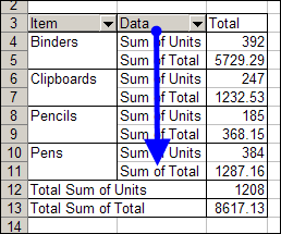
If you wanted the data headings arranged horizontally, you could drag the data button in the Column area.
Here is the same pivot table, with horizontal data headings.
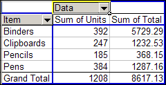
Vertical Data in Excel 2010 Pivot Table
Pivot tables changed quite a bit in Excel 2007, and the default layout for multiple data fields is now horizontal. Using the same data, this is the default layout in Excel 2010.
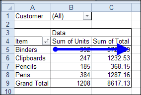
If you want to change the data to a vertical layout, you can drag the Values button in the Pivot Table Field List, from the Column Labels area to the Row Labels area.
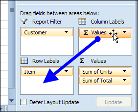
Usually, the Values button would be positioned below the other fields in the Row Labels area.
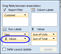
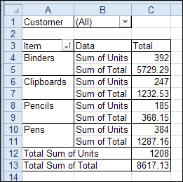
After you move the Values label, the data fields will be rearranged, and they will show vertically, with headings in the Row Labels area.
Watch the Excel 2010 Data Layout Video
To see the steps for rearranging the data in Excel 2010, please watch this short video tutorial.
_____________

Good to know. I was wondering about the default layout change in Excel 2007, and couldn’t figure out how to get back to the Excel 2003 format. Thanks for sharing.