Fix Pivot Table Source Data For Better Results

When you are setting up your source data for an Excel pivot table, there are a few data layout guidelines that will help you create the best possible pivot table. Get it right, and you won’t have to fix Pivot Table source data later!

Sometimes you get data that isn’t well suited for creating a pivot table, like the example shown below. It has a column for each month, and the sales amounts are spread over those 12 columns.

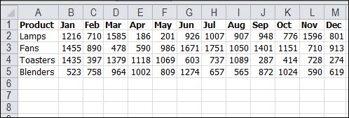
When you create a pivot table, there are 12 value fields – one for each month – and you would have to create a calculated field to see an annual total.

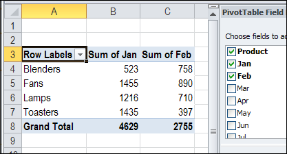
Fix Pivot Table Source Data

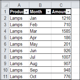
Instead of a separate column for each month, the pivot table source data should have a single column for the sales amounts. In the adjacent columns, you can enter the product name and month name for each amount.

You could manually fix Pivot Table source data, or write an Excel macro to do the job for you, so it looks like the table shown below.

With this 3-column Excel table, you can easily create a flexible pivot table, and focus of specific items or months.

Rearrange the Data Without Macros

Instead of manually rearranging the data, or writing a macro, you can use a pivot table trick to change the 13-column data into a normalized 3-column table. Follow these steps, to quickly fix Pivot Table source data:

1. Select a cell in the 13-column table, and press Alt+D, and then press P, to open the PivotTable and PivotChart Wizard
2. In Step 1, select Multiple Consolidation Ranges, and then click Next.
3. In Step 2a, select I Will Create The Page Fields, and then click Next.
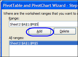
4. In Step 2b, click in the Range box, and on the worksheet, select the entire table, including the headings, and then click Add.
   • 
5. Leave the other settings at their defaults, and click Finish.
6. A new sheet is added to the workbook, with a pivot table
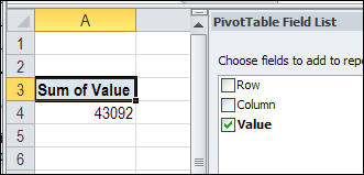
7. In the PivotTable Field List, remove the check marks from the Row and Column fields, so only the Grand Total for Value is left.
   • 
8. Double-click the Grand Total cell, (cell A4 in the screen shot above), to create a new sheet, with the pivot table’s data in 3 columns.
9. Then, rename the heading cells as Product, Month, and Amount.
   • 

Build a New Pivot Table

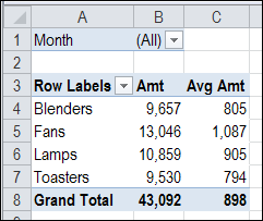
Now that the source data is normalized, in a 3-column table instead of 13 columns, you can insert your final pivot table, based on the rearranged data.

With the amounts in a single columns, it’s easy to create totals, and use other summary functions, such as Average.

Download the Sample Workbook

To test the multiple consolidation ranges technique, you can download the sample workbook from my Contextures website. Go to the Fix Pivot Source Data page, and look in the Download section.

The file is in xlsx format, and is zipped. There are no macros in the file.

Watch the Pivot Table Trick Video

To see the steps for using a multiple consolidation ranges pivot table, to rearrange your pivot table source data, watch this Excel video tutorial.

It also shows the steps for this technique, if there are two or more columns with labels.

________________

Save